Introduction to tsgp

library(tsgp)
library(ggplot2)

Purpose

tsgp is a lightweight package for modelling univariate time-series data with Gaussian processes (GP). It is important to remember that using a GP for time series basically converts the problem from one of modelling a generative process (e.g., if we used an ARIMA model) to that of essentially a curve-fitting exercise. GPs are a Bayesian method, so if you are unfamiliar with Bayesian inference, please go check out some resources on that, such as this great video by Richard McElreath. Essentially, the key bits to remember for this post is that in Bayesian inference, we are interested in the posterior distribution, which is proportional to the product of the prior (our beliefs about an event before seeing the data) and the likelihood (the probability of the data given model parameters).

If you would like a deeper treatment of how GPs can model time-series data, please see this post.

Generating some data

We are going to simulate some time series data with temporal dynamics that are commonly encountered in applied settings. Specifically, we are going to generate a noisy sine wave (i.e., to emulate periodic or seasonal data) with a linearly increasing trend:

set.seed(123)
y <- 3 * sin(2 * seq(0, 4 * pi, length.out = 100)) + runif(100) * 2
trend <- 0.08 * seq(from = 1, to = 100, by = 1)
y <- y + trend
tmp <- data.frame(timepoint = 1:length(y), y = y)
x1 <- 1:length(y)

# Draw plot

ggplot(data = tmp) +
  geom_point(aes(x = timepoint, y = y), colour = "black") +
  geom_line(aes(x = timepoint, y = y), colour = "black") +
  labs(x = "Timepoint",
       y = "Values") +
  theme_bw()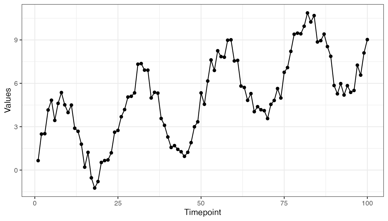

Package functionality

Covariance functions

tsgp contains several covariance functions (coded in C++ for efficiency). All of them return an object of class GPCov (which is just a matrix but with a new inherited class that allows us to make use of R’s generic functions).

Exponentiated quadratic

\[ k(x, x') = \text{exp} \left( -\frac{1}{2\sigma^{2}}||x - x'||^{2} \right) \]

In tsgp, cov_exp_quad takes the following arguments:

xa — vector of values
xb — vector of values
sigma — scalar denoting the variance. Defaults to 1
l — scalar denoting the lengthscale. Defaults to 1

We can produce two types of plots for GPCov objects by calling the plot() generic. The first is a plot of samples from the prior distribution, which we specify by setting type = "prior", passing in the input vector (x2 in this example), and setting the number of samples to draw through the argument k. Here is an example:

x2 <- seq(from = -2, to = 2, length.out = 100)
mat_exp_quad <- cov_exp_quad(x2, x2, 1, 1)
plot(mat_exp_quad, x2, type = "prior", k = 5)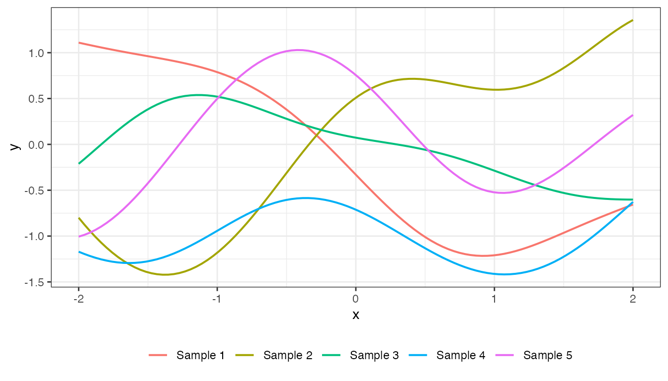

The second is a plot of the covariance matrix represented as a heatmap:

plot(mat_exp_quad, type = "matrix")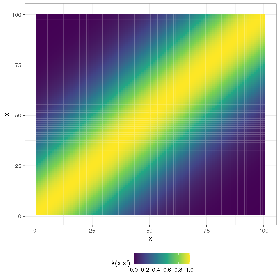

Rational quadratic

\[ k(x, x') = \sigma^{2} \left( 1 + \frac{||x - x'||^{2}}{2\alpha \mathcal{l}^{2}} \right)^{-\alpha} \]

In tsgp, cov_rat_quad takes the following arguments:

xa — vector of values
xb — vector of values
sigma — scalar denoting the variance. Defaults to 1
alpha — scalar \(>0\) denoting the mixing coefficient. Defaults to 1
l — scalar denoting the lengthscale. Defaults to 1

mat_rat_quad <- cov_rat_quad(x2, x2, 1, 1, 1)
plot(mat_rat_quad, x2, type = "prior", k = 5)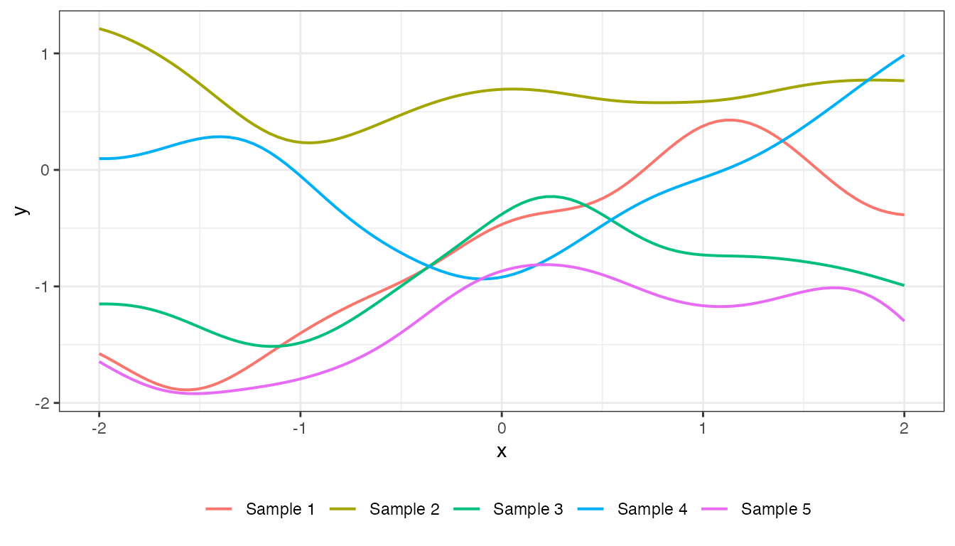

plot(mat_rat_quad, type = "matrix")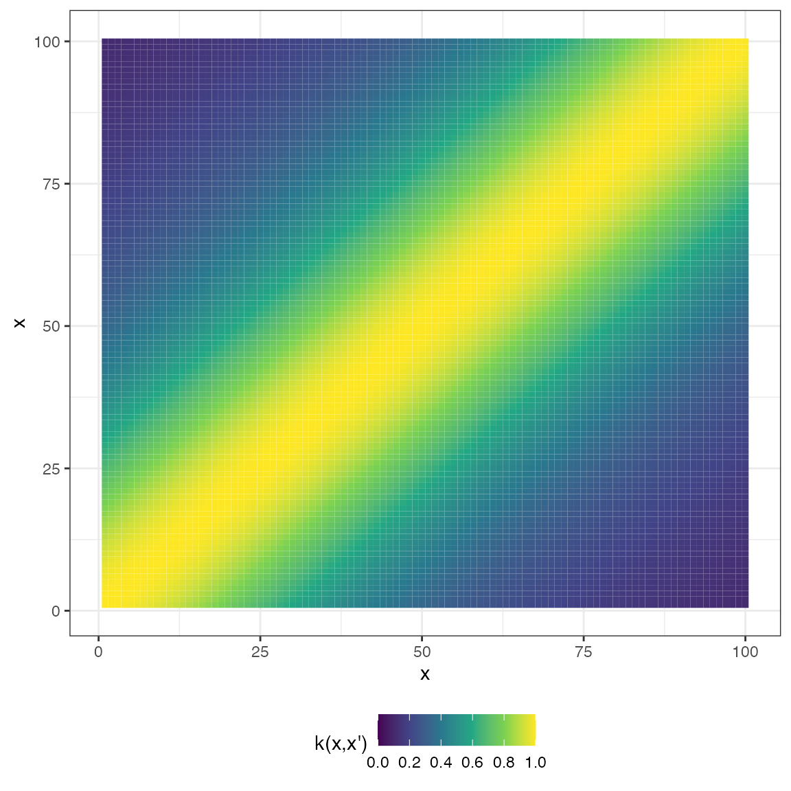

Periodic

\[ k(x, x') = \sigma^{2} \text{exp} \left( -\frac{2}{\mathcal{l}^{2}}\text{sin}^{2} \left( \pi\frac{|x - x'|}{p} \right) \right) \]

In tsgp, cov_periodic takes the following arguments:

xa — vector of values
xb — vector of values
sigma — scalar denoting the variance. Defaults to 1
l — scalar denoting the lengthscale. Defaults to 1
p — scalar denoting the period. Defaults to 1

mat_periodic <- cov_periodic(x2, x2, 1, 1, 1)
plot(mat_periodic, x2, type = "prior", k = 5)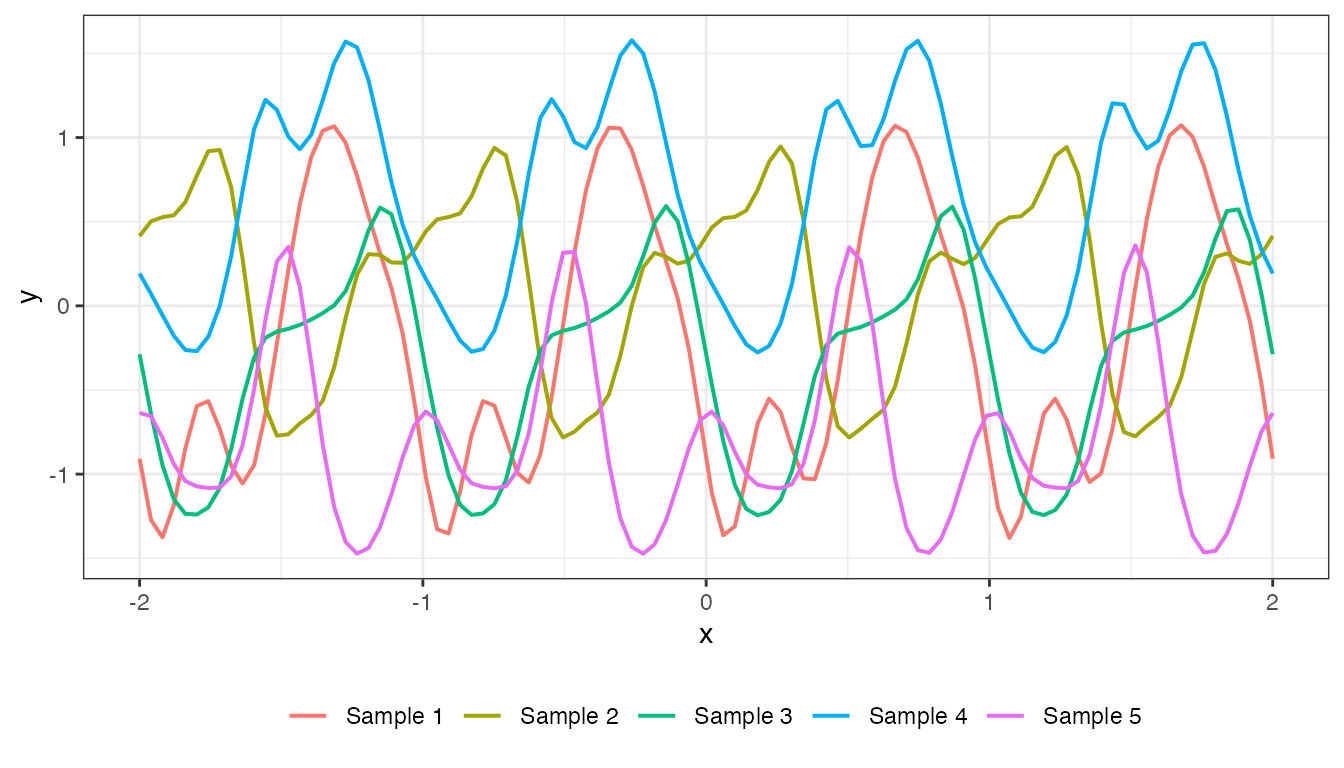

plot(mat_periodic, type = "matrix")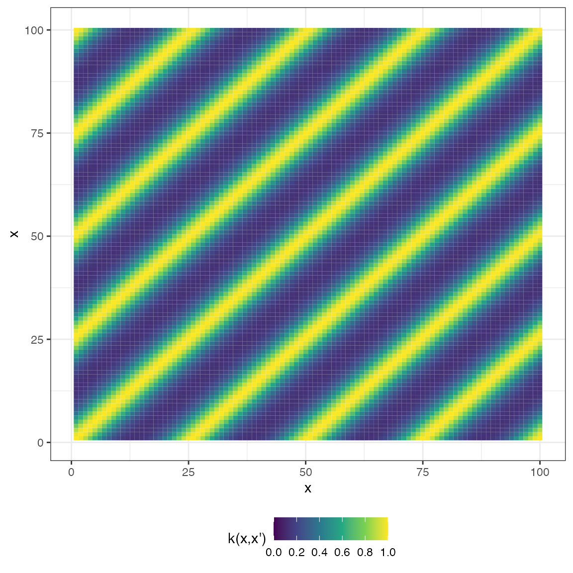

Linear

\[ k(x,x') = \sigma^{2}_{b} + \sigma^{2}_{v} (x−c)(x'−c) \]

In tsgp, cov_linear takes the following arguments:

xa — vector of values
xb — vector of values
sigma_b — scalar denoting the constant variance. Defaults to 1
sigma_v — scalar denoting the constant variance. Defaults to 1
c — scalar denoting the offset. Defaults to 1

mat_linear <- cov_linear(x2, x2, 1, 1, 1)
plot(mat_linear, x2, type = "prior", k = 5)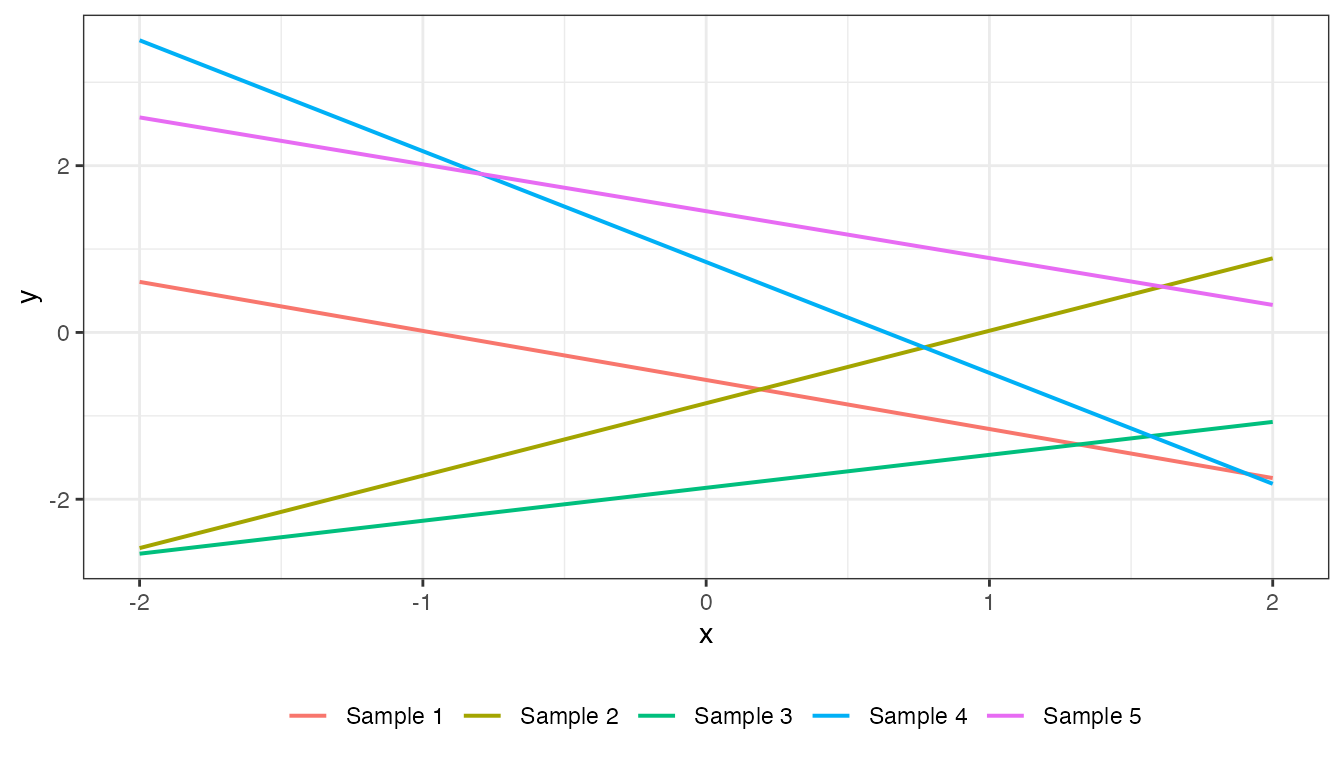

plot(mat_linear, type = "matrix")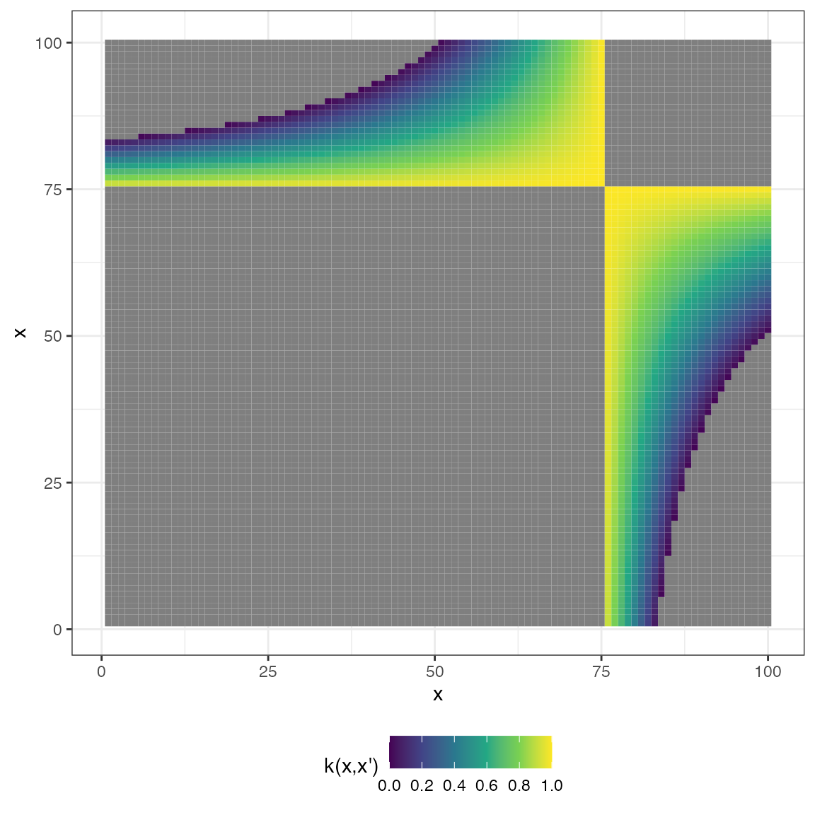

White noise

\[ k(x, x') = \sigma^{2}I_{n} \]

In tsgp, noise is handled within the core GP function since it only applies to the covariance matrix between observations. The GP function is discussed later in this vignette.

However, for visual comparison to the other covariance functions, here is what it looks like:

cov_noise <- function(x, sigma = 0.5){
  X <- sigma * diag(length(x))
  X <- structure(X, class = c("GPCov", "matrix"))
  return(X)
}

mat_noise <- cov_noise(x2, 0.5)
plot(mat_noise, x2, type = "prior", k = 5)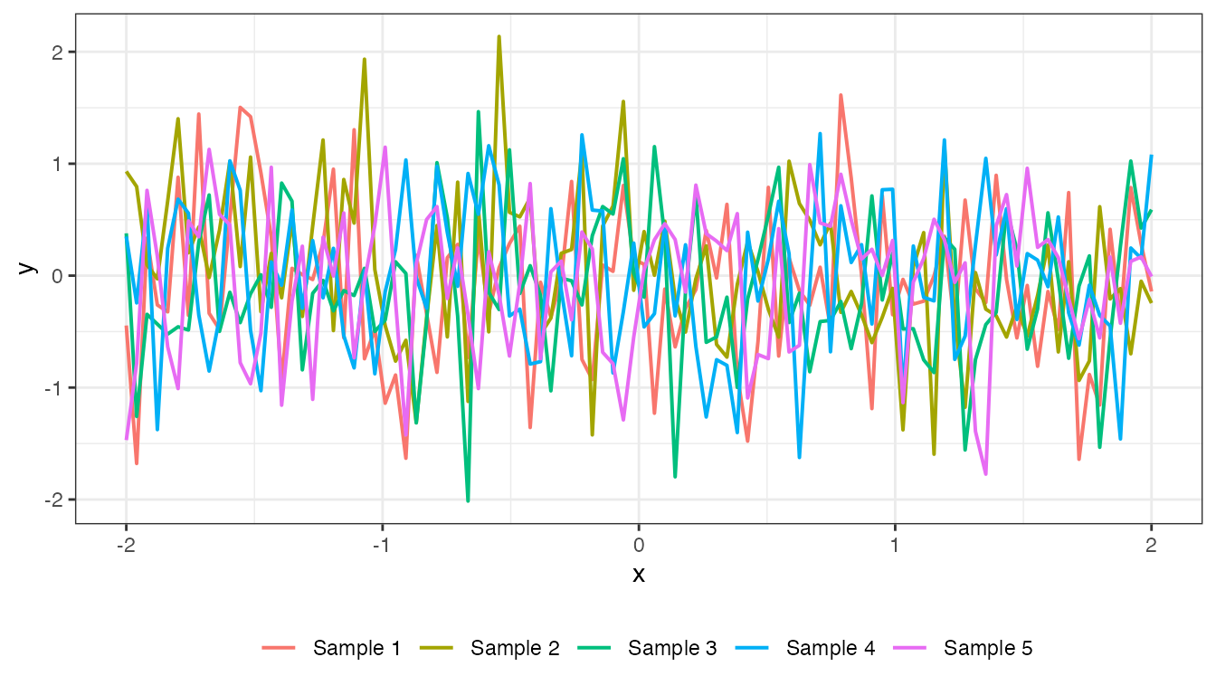

plot(mat_noise, type = "matrix")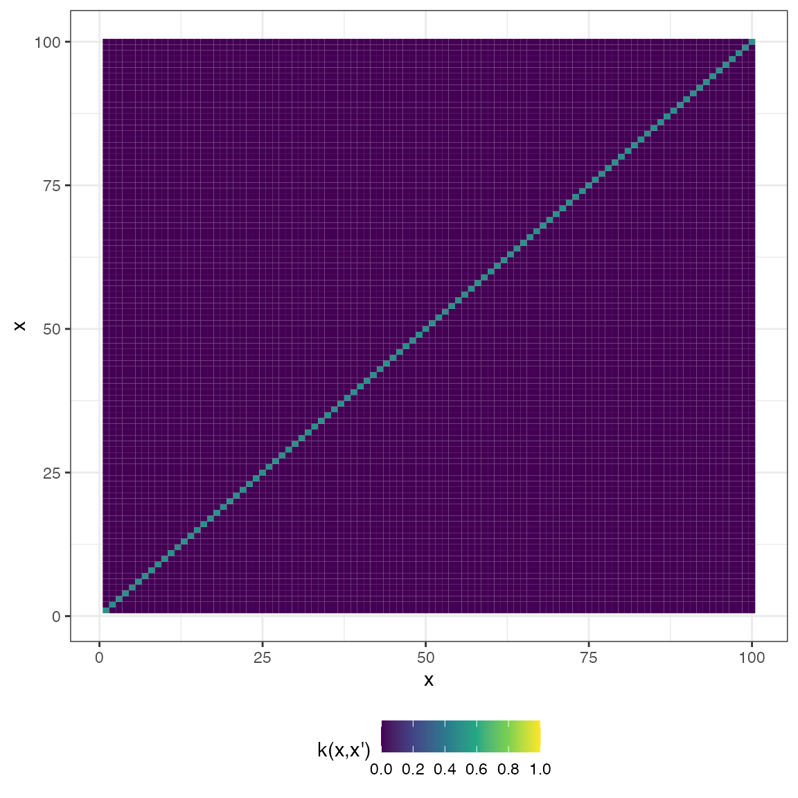

Combining covariance functions

Often in time-series analysis we need our models to capture multiple different statistical dynamics simultaneusly, such as trend, seasonality, and noise. It is quite easy to define a custom composite kernel function which either sums or multiplies different kernels:

CovSum <- function(xa, xb, sigma_1 = 1, sigma_2 = 1, l_1 = 1, l_2 = 1, p = 1){
  X <- cov_exp_quad(xa, xb, sigma_1, l_1) + 
    cov_periodic(xa, xb, sigma_2, l_2, p)
  
  X <- structure(X, class = c("GPCov", "matrix"))
  return(X)
}

Model fitting

The core function in tsgp to calculate the posterior mean vector and covariance matrix is GP. GP returns an object of class TSGP which is a list of the input data, the posterior mean vector, and the posterior covariance matrix. GP takes the following arguments:

x — vector of input data
xprime — vector of data points to predict values for
y — vector of values to learn from
covfun — function specifying the covariance
noise — scalar denoting the noise variance to add to the \((x, x)\) covariance matrix of observations. Defaults to 0 for no noise modelling
... — hyperparameters to be passed to cov_function

Here is an example for a model which predicts values for a set of uniformally-distributed time points over the \([1-100]\) domain:

mod <- GP(x1, seq(from = 1, to = 100, by = 5), y, CovSum, noise = 0.8,
           sigma_1 = 5, sigma_2 = 1, l_1 = 75, l_2 = 1, p = 25)

names(mod)
#> [1] "x"      "xprime" "y"      "mu"     "Sigma"

Model visualisation

We can easily visualise draws from the posterior distribution by calling plot() on a TSGP object. The plot() generic for TSGP takes only three arguments:

x — TSGP model object
prob — desired credible interval probability level. Defaults to 0.95 for a \(95\%\) credible interval
draws — number of posterior draws to summarise over. Defaults to \(100\)

Here is an example:

plot(mod, 0.95, 100)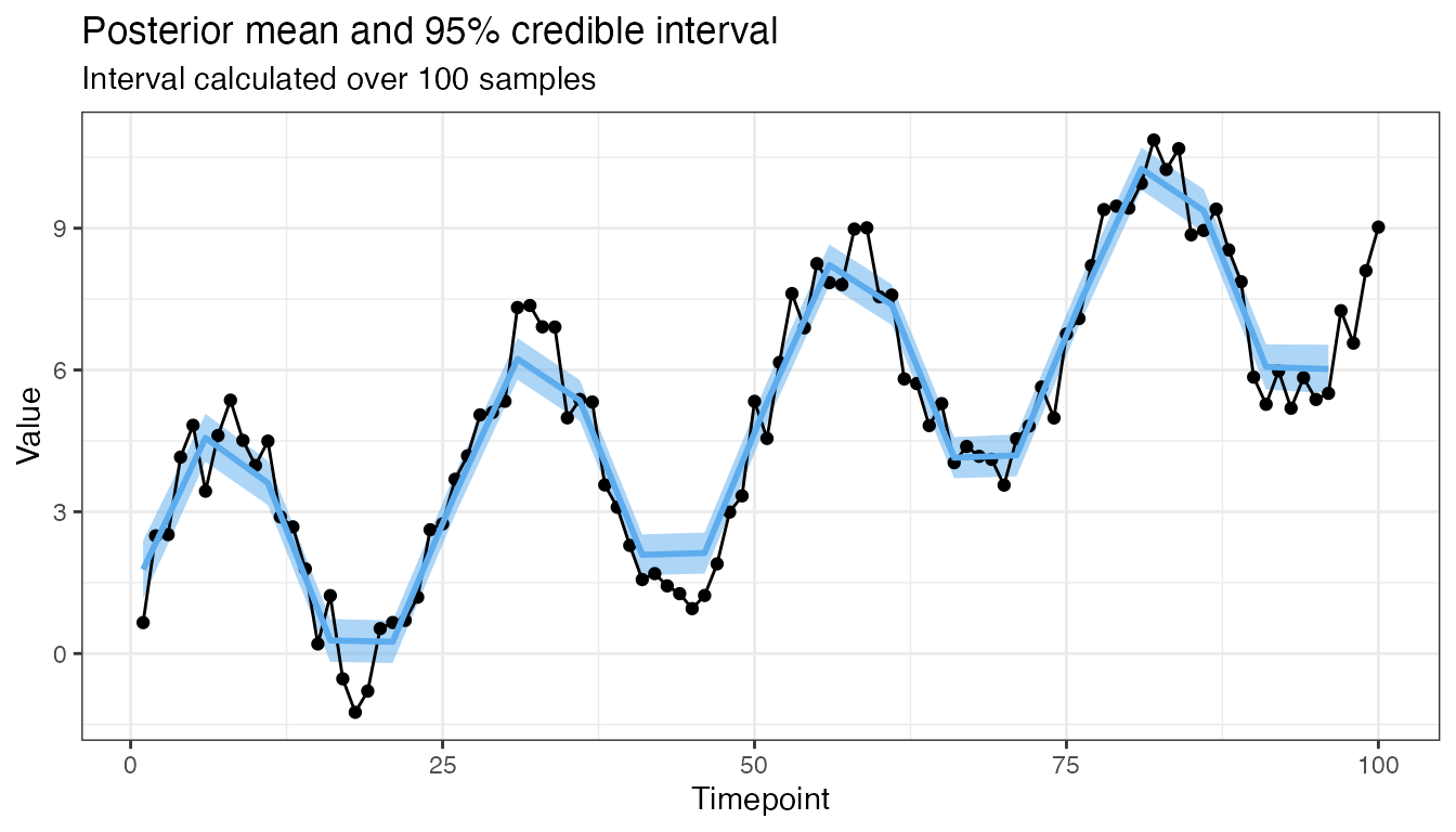

Here is another for a model which predicts for all time points but with \(1000\) draws:

mod2 <- GP(x1, x1, y, CovSum, 0.8,
           sigma_1 = 5, sigma_2 = 1, l_1 = 75, l_2 = 1, p = 25)

plot(mod2, 0.95, 1000)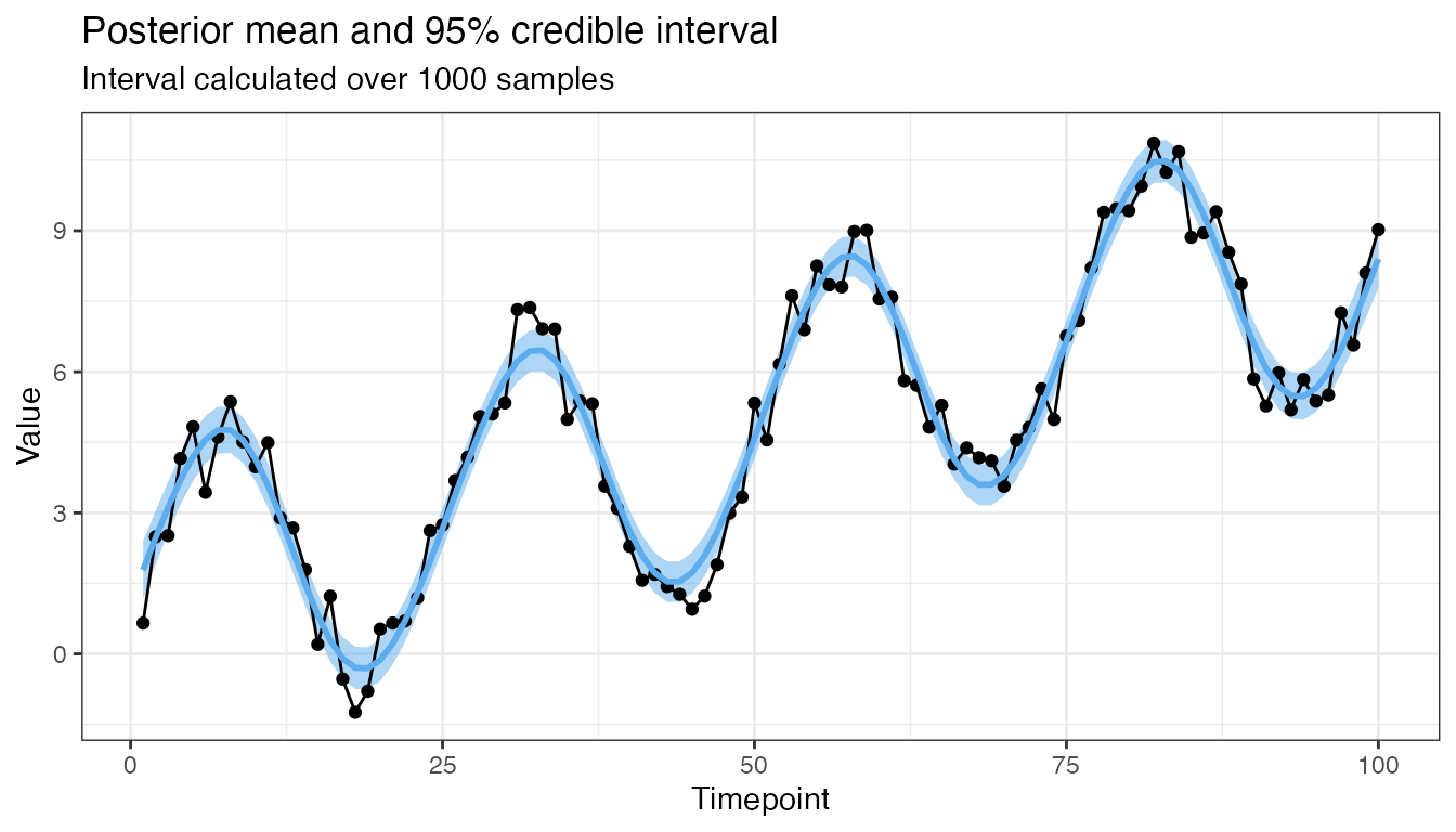

Need more uncertainty?

mod3 <- GP(x1, x1, y, CovSum, noise = 1.75,
           sigma_1 = 5, sigma_2 = 1, l_1 = 75, l_2 = 1, p = 25)

plot(mod3, 0.95, 1000)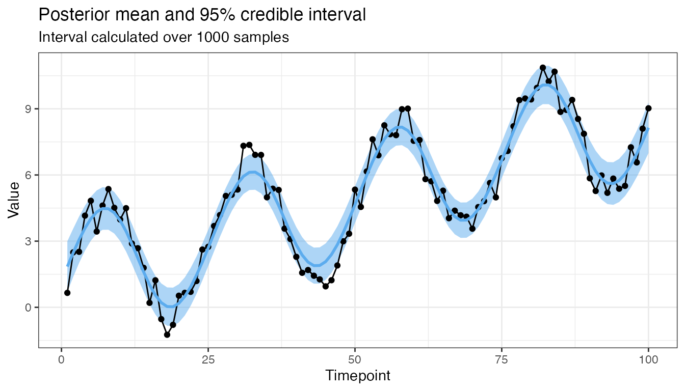

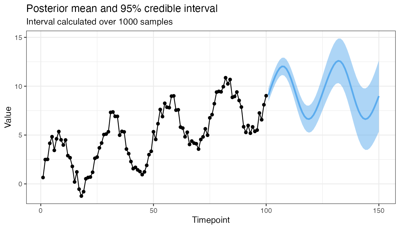
What about a short-range forecast?

mod4 <- GP(x1, 101:150, y, CovSum, 0.8,
           sigma_1 = 5, sigma_2 = 1, l_1 = 75, l_2 = 1, p = 25)

plot(mod4, 0.95, 1000)

Trent Henderson

2024-05-06